PROJECT INFORMATION

Graphic Name: What is the impact of the hydronic configuration on the performance of a hybrid heat production system?

Submitted by: Freek Van Riet

Firm Name: University of Antwerp

Other contributors or acknowledgements (optional)

What tools did you use to create the graphic?

• Matlab

What kind of graphic is this?

Primary Inputs: The inputs required to create this extended type of Load Duration Curve (LDC) are heat loads throughout a year of an hydronic heat production system with its different components. The loads can originate from both measurements and simulations. In this simulation-based case the yearly loads of three components were taken as input: a cogeneration device (CHP), a storage tank and an auxiliary boiler.

Primary Outputs:

1) the total heat load of the building, which is the sum of the loads of the three components (CHP, tank and boiler), sorted in descending order = conventional LDC.

2) the heat loads of the three components separately, corresponding to the descending order of the total heat load.

3) the load duration curve of the CHP itself.

4) areas indicate total heat produced (or charged/discharged) by each component.

5) upper outputs are given for both the ‘expected’ behavior (i.e. what one can expect of a properly working installation) and the real ones for different design concepts.

6) in the graphs, three levels of load can be distinguished: peak, base and part load.

GRAPHIC INFORMATION

What are we looking at?

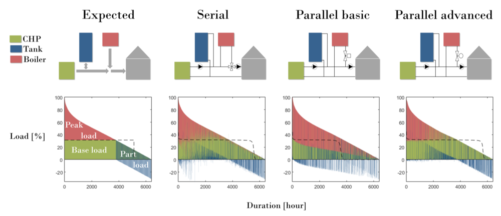
Most people who design heating systems of buildings are familiar with a ‘load duration curve’: it is a common graphical representation of the heat demand of a building. But did you know that in the same graphic much more information can be shown, to indicate the performance of the heat production system in the blink of an eye? Especially when different heat production components are combined into a ‘hybrid heat production system’, this is beneficial. In the four schemes (upper part of figure), a hybrid production system with its possible designs of hydronic configurations are shown as an example. The first, ‘expected’, explains the heat flows in general and in the three following ones particular design options for the hydronic configuration are shown. In the lower part of the figure, the load duration curves including the loads of the three components are shown, corresponding to the upper schemes. This is the part of the figure that is automatically generated and is proposed here as ‘the fingerprint of a hybrid heat production system’. The x-axis shows the duration in hours and the y-axis the loads, relative to the maximum load of the building. In the reference results (‘expected’) three levels of heat load are distinguished, according to how an in-theory-proper-working installation would perform: -the base heat load is provided by the CHP -the heat demand higher than the CHPs load (dotted line=load duration curve of CHP itself) is covered by an auxiliary boiler – at heat demands of the building lower than the heat load of the CHP, two possible situations can occur. First, the CHP is on and the heat that is not consumed by the building is stored in the tank. Second, the CHP is off and the stored heat is discharged from the tank to heat the building. If the behaviour of the three hydronic configurations are compared with this expected behaviour, some conclusions can be drawn, such as: – for the ‘parallel basic’-configuration, a part of the base load is covered by the boiler instead of the CHP: the figure clearly shows that the hydronics fail, causing the CHP to operate less hours than expected. This configuration should be excluded from the possible designs. -for the two other hydronic configurations the tank can cover partially the base load, for which the CHP can produce more heat than expected.

How did you make the graphic?

An algorithms post-processes the data of full year simulations. The total heat demand is calculated as the some of the loads of the three components, and that total demand is sorted in descending order. Then, the different loads are plotted as stacked areas.

What specific investigation questions led to the production of this graphic?

– How to evaluate hybrid heat production systems?

– How should a CHP device be integrated in the heat production system of a building?

– What is the effect of buffer tank volume on CHP operation?

– How to ensure the priority of operation of the CHP above that of an auxiliary heater?

How does this graphic fit into the larger design investigations and what did you learn from producing the graphic?

This type of LDC shows how a particular hydronic configuration influences the operation of a heat production system. Because it is compared with an in-theory-proper-working installation, it enables to detect faults and benefits of the configuration. By creating these figures I learned about the disadvantages of each configuration, without necessarily looking into the detailed dynamic simulation data.

What was successful and/or unique about the graphic in how it communicates information?

Load Duration Curves (LDC) are widely used to communicate about the heat demand of a building. In this extended type of LDC, the load of each single heat-producing component is added, thereby providing much more insight. Indeed, not only the heat demand of the building can be seen, also the way this heat is delivered or stored is shown. Because LDCs as such are familiar, these graphics are easy accessible for both researchers and engineers working in the field of heating.

What would you have done differently with the graphic if you had more time/fee?

In the end, designers or owners are interested in fuel consumption and the resulting costs, and not necessarily in heat as such. The relation between both are, of course, the efficiencies of all the components, which are not shown in these figures. Hence, extra graphics showing the efficiencies or fuel consumption would be interesting, especially to incorporate the effect of temperature levels in the installation.